Example
To illustrate the trend fitting functionality of i2extras we will use the simulated Ebola Virus Disease (EVD) outbreak data from the outbreaks package.
Loading relevant packages and data
library(outbreaks)
library(i2extras)
#> Loading required package: incidence2
#> Loading required package: grates
library(ggplot2)

raw_dat <- ebola_sim_clean$linelist
For this example we will restrict ourselves to the first 20 weeks of data:
dat <- incidence(
    raw_dat,
    date_index = "date_of_onset",
    interval = "week",
    groups = "gender"
)[1:20, ]
dat
#> # incidence:  20 x 4
#> # count vars: date_of_onset
#> # groups:     gender
#>    date_index gender count_variable count
#>  * <isowk>    <fct>  <chr>          <int>
#>  1 2014-W15   f      date_of_onset      1
#>  2 2014-W16   m      date_of_onset      1
#>  3 2014-W17   f      date_of_onset      4
#>  4 2014-W17   m      date_of_onset      1
#>  5 2014-W18   f      date_of_onset      4
#>  6 2014-W19   f      date_of_onset      9
#>  7 2014-W19   m      date_of_onset      3
#>  8 2014-W20   f      date_of_onset      7
#>  9 2014-W20   m      date_of_onset     10
#> 10 2014-W21   f      date_of_onset      8
#> 11 2014-W21   m      date_of_onset      7
#> 12 2014-W22   f      date_of_onset      9
#> 13 2014-W22   m      date_of_onset     10
#> 14 2014-W23   f      date_of_onset     13
#> 15 2014-W23   m      date_of_onset     10
#> 16 2014-W24   f      date_of_onset      7
#> 17 2014-W24   m      date_of_onset     14
#> 18 2014-W25   f      date_of_onset     15
#> 19 2014-W25   m      date_of_onset     15
#> 20 2014-W26   f      date_of_onset     12
plot(dat, angle = 45, border_colour = "white")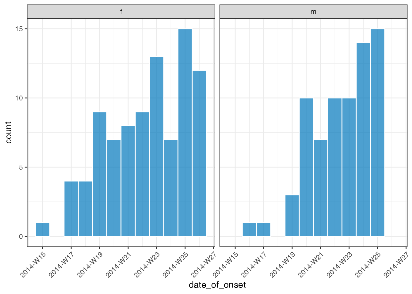
Modeling incidence
We can use fit_curve() to fit the data with either a poisson or negative binomial regression model. The output from this will be a nested object with class incidence2_fit which has methods available for both automatic plotting and the calculation of growth (decay) rates and doubling (halving) times.
out <- fit_curve(dat, model = "poisson", alpha = 0.05)
out
#> # A tibble: 2 × 9
#> count_varia…¹ gender data model estimates fitti…² fitti…³ predi…⁴ predi…⁵
#> <chr> <fct> <list<t> <lis> <list> <list> <list> <list> <list>
#> 1 date_of_onset f [11 × 2] <glm> <trndng_p> <NULL> <NULL> <NULL> <NULL>
#> 2 date_of_onset m [9 × 2] <glm> <trndng_p> <NULL> <NULL> <NULL> <NULL>
#> # … with abbreviated variable names ¹count_variable, ²fitting_warning,
#> # ³fitting_error, ⁴prediction_warning, ⁵prediction_error
plot(out, angle = 45, border_colour = "white")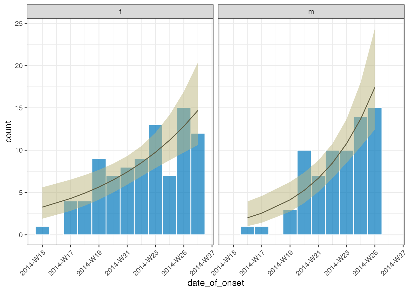
growth_rate(out)
#> # A tibble: 2 × 10
#> count_varia…¹ gender model r r_lower r_upper growt…² time time_…³ time_…⁴
#> <chr> <fct> <lis> <dbl> <dbl> <dbl> <chr> <dbl> <dbl> <dbl>
#> 1 date_of_onset f <glm> 0.137 0.0698 0.206 doubli… 5.07 3.36 9.93
#> 2 date_of_onset m <glm> 0.240 0.146 0.341 doubli… 2.89 2.03 4.75
#> # … with abbreviated variable names ¹count_variable, ²growth_or_decay,
#> # ³time_lower, ⁴time_upperTo unnest the data we can use unnest() (a function that has been reexported from the tidyr package.
unnest(out, estimates)
#> # A tibble: 20 × 15
#> count_v…¹ gender data model count date_…² estim…³ lower…⁴ upper…⁵ lower…⁶
#> <chr> <fct> <list<t> <lis> <int> <isowk> <dbl> <dbl> <dbl> <dbl>
#> 1 date_of_… f [11 × 2] <glm> 1 2014-W… 3.27 1.90 5.61 0
#> 2 date_of_… f [11 × 2] <glm> 4 2014-W… 4.30 2.83 6.52 0
#> 3 date_of_… f [11 × 2] <glm> 4 2014-W… 4.93 3.44 7.06 0
#> 4 date_of_… f [11 × 2] <glm> 9 2014-W… 5.65 4.15 7.68 1
#> 5 date_of_… f [11 × 2] <glm> 7 2014-W… 6.47 4.99 8.40 1
#> 6 date_of_… f [11 × 2] <glm> 8 2014-W… 7.42 5.92 9.31 2
#> 7 date_of_… f [11 × 2] <glm> 9 2014-W… 8.51 6.90 10.5 2
#> 8 date_of_… f [11 × 2] <glm> 13 2014-W… 9.75 7.88 12.1 3
#> 9 date_of_… f [11 × 2] <glm> 7 2014-W… 11.2 8.82 14.2 4
#> 10 date_of_… f [11 × 2] <glm> 15 2014-W… 12.8 9.72 16.9 4
#> 11 date_of_… f [11 × 2] <glm> 12 2014-W… 14.7 10.6 20.4 5
#> 12 date_of_… m [9 × 2] <glm> 1 2014-W… 2.01 1.02 3.95 0
#> 13 date_of_… m [9 × 2] <glm> 1 2014-W… 2.56 1.43 4.59 0
#> 14 date_of_… m [9 × 2] <glm> 3 2014-W… 4.13 2.73 6.24 0
#> 15 date_of_… m [9 × 2] <glm> 10 2014-W… 5.25 3.75 7.36 1
#> 16 date_of_… m [9 × 2] <glm> 7 2014-W… 6.67 5.07 8.79 1
#> 17 date_of_… m [9 × 2] <glm> 10 2014-W… 8.48 6.69 10.8 2
#> 18 date_of_… m [9 × 2] <glm> 10 2014-W… 10.8 8.50 13.7 3
#> 19 date_of_… m [9 × 2] <glm> 14 2014-W… 13.7 10.4 18.0 5
#> 20 date_of_… m [9 × 2] <glm> 15 2014-W… 17.4 12.4 24.4 6
#> # … with 5 more variables: upper_pi <dbl>, fitting_warning <list>,
#> # fitting_error <list>, prediction_warning <list>, prediction_error <list>,
#> # and abbreviated variable names ¹count_variable, ²date_index, ³estimate,
#> # ⁴lower_ci, ⁵upper_ci, ⁶lower_pifit_curve() also works nicely with grouped incidence2 objects. In this situation, we return a nested tibble with some additional columns that indicate whether there has been a warning or error during the fitting or prediction stages.
grouped_dat <- incidence(
raw_dat,
date_index = "date_of_onset",
interval = "week",
groups = "hospital"
)[1:120, ]
grouped_dat
#> # incidence: 120 x 4
#> # count vars: date_of_onset
#> # groups: hospital
#> date_index hospital count_variable count
#> * <isowk> <fct> <chr> <int>
#> 1 2014-W15 Military Hospital date_of_onset 1
#> 2 2014-W16 Connaught Hospital date_of_onset 1
#> 3 2014-W17 NA date_of_onset 2
#> 4 2014-W17 other date_of_onset 3
#> 5 2014-W18 NA date_of_onset 1
#> 6 2014-W18 Connaught Hospital date_of_onset 1
#> 7 2014-W18 Princess Christian Maternity Hospital (PCMH) date_of_onset 1
#> 8 2014-W18 Rokupa Hospital date_of_onset 1
#> 9 2014-W19 NA date_of_onset 1
#> 10 2014-W19 Connaught Hospital date_of_onset 3
#> # … with 110 more rows
out <- fit_curve(grouped_dat, model = "poisson", alpha = 0.05)
out
#> # A tibble: 6 × 9
#> count_vari…¹ hospi…² data model estimates fitti…³ fitti…⁴ predi…⁵ predi…⁶
#> <chr> <fct> <list<t> <lis> <list> <list> <list> <list> <list>
#> 1 date_of_ons… Connau… [22 × 2] <glm> <trndng_p> <NULL> <NULL> <NULL> <NULL>
#> 2 date_of_ons… Milita… [21 × 2] <glm> <trndng_p> <NULL> <NULL> <NULL> <NULL>
#> 3 date_of_ons… other [20 × 2] <glm> <trndng_p> <NULL> <NULL> <NULL> <NULL>
#> 4 date_of_ons… Prince… [17 × 2] <glm> <trndng_p> <NULL> <NULL> <NULL> <NULL>
#> 5 date_of_ons… Rokupa… [18 × 2] <glm> <trndng_p> <NULL> <NULL> <NULL> <NULL>
#> 6 date_of_ons… NA [22 × 2] <glm> <trndng_p> <NULL> <NULL> <NULL> <NULL>
#> # … with abbreviated variable names ¹count_variable, ²hospital,
#> # ³fitting_warning, ⁴fitting_error, ⁵prediction_warning, ⁶prediction_error
# plot with a prediction interval but not a confidence interval
plot(out, ci = FALSE, pi=TRUE, angle = 45, border_colour = "white")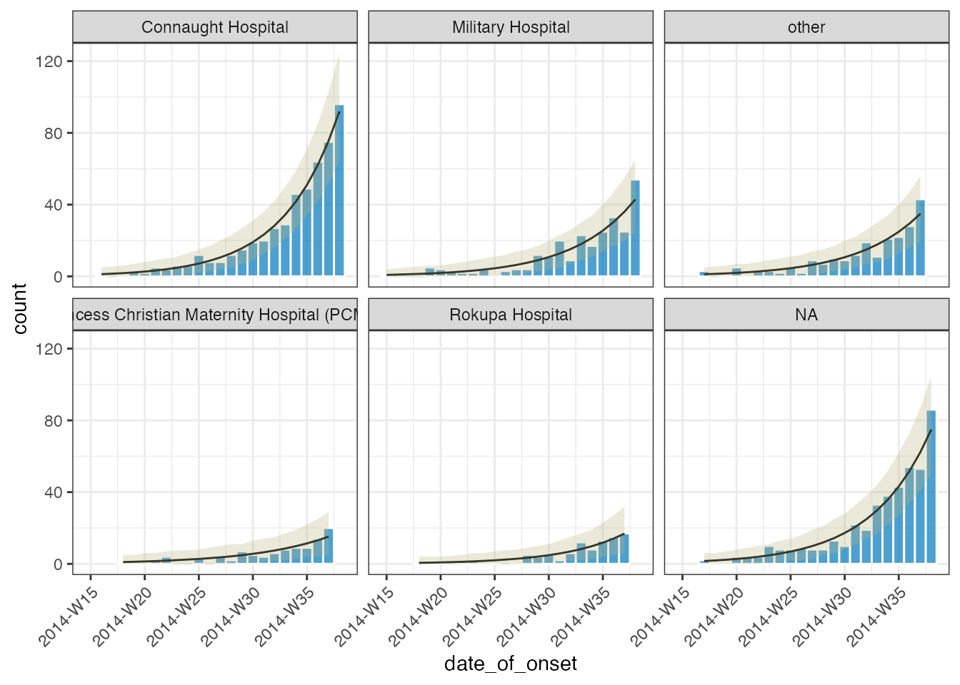
growth_rate(out)
#> # A tibble: 6 × 10
#> count_vari…¹ hospi…² model r r_lower r_upper growt…³ time time_…⁴ time_…⁵
#> <chr> <fct> <lis> <dbl> <dbl> <dbl> <chr> <dbl> <dbl> <dbl>
#> 1 date_of_ons… Connau… <glm> 0.197 0.177 0.217 doubli… 3.53 3.20 3.92
#> 2 date_of_ons… Milita… <glm> 0.173 0.147 0.200 doubli… 4.00 3.46 4.71
#> 3 date_of_ons… other <glm> 0.170 0.141 0.200 doubli… 4.09 3.46 4.92
#> 4 date_of_ons… Prince… <glm> 0.142 0.101 0.188 doubli… 4.87 3.70 6.87
#> 5 date_of_ons… Rokupa… <glm> 0.178 0.133 0.228 doubli… 3.89 3.04 5.22
#> 6 date_of_ons… NA <glm> 0.184 0.164 0.205 doubli… 3.77 3.39 4.24
#> # … with abbreviated variable names ¹count_variable, ²hospital,
#> # ³growth_or_decay, ⁴time_lower, ⁵time_upperWe provide helper functions, is_ok(), is_warning() and is_error() to help filter the output as necessary.
out <- fit_curve(grouped_dat, model = "negbin", alpha = 0.05)
is_warning(out)
#> # A tibble: 5 × 7
#> count_variable hospital data model estimates fitti…¹ predi…²
#> <chr> <fct> <list<t> <list> <list> <list> <list>
#> 1 date_of_onset Connaught Hospital [22 × 2] <negbin> <trndng_p> <chr> <NULL>
#> 2 date_of_onset other [20 × 2] <negbin> <trndng_p> <chr> <NULL>
#> 3 date_of_onset Princess Christia… [17 × 2] <negbin> <trndng_p> <chr> <NULL>
#> 4 date_of_onset Rokupa Hospital [18 × 2] <negbin> <trndng_p> <chr> <NULL>
#> 5 date_of_onset NA [22 × 2] <negbin> <trndng_p> <chr> <NULL>
#> # … with abbreviated variable names ¹fitting_warning, ²prediction_warning
unnest(is_warning(out), fitting_warning)
#> # A tibble: 10 × 7
#> count_variable hospital data model estimates fitti…¹ predi…²
#> <chr> <fct> <list<t> <list> <list> <chr> <list>
#> 1 date_of_onset Connaught Hospit… [22 × 2] <negbin> <trndng_p> iterat… <NULL>
#> 2 date_of_onset Connaught Hospit… [22 × 2] <negbin> <trndng_p> iterat… <NULL>
#> 3 date_of_onset other [20 × 2] <negbin> <trndng_p> iterat… <NULL>
#> 4 date_of_onset other [20 × 2] <negbin> <trndng_p> iterat… <NULL>
#> 5 date_of_onset Princess Christi… [17 × 2] <negbin> <trndng_p> iterat… <NULL>
#> 6 date_of_onset Princess Christi… [17 × 2] <negbin> <trndng_p> iterat… <NULL>
#> 7 date_of_onset Rokupa Hospital [18 × 2] <negbin> <trndng_p> iterat… <NULL>
#> 8 date_of_onset Rokupa Hospital [18 × 2] <negbin> <trndng_p> iterat… <NULL>
#> 9 date_of_onset NA [22 × 2] <negbin> <trndng_p> iterat… <NULL>
#> 10 date_of_onset NA [22 × 2] <negbin> <trndng_p> iterat… <NULL>
#> # … with abbreviated variable names ¹fitting_warning, ²prediction_warningRolling average
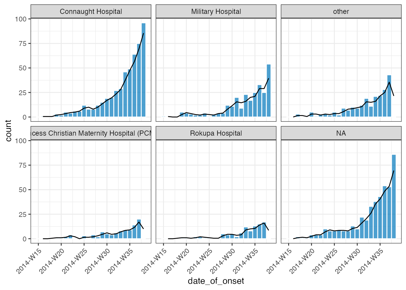
We can add a rolling average, across current and previous intervals, to an incidence2 object with the add_rolling_average() function:
ra <- add_rolling_average(grouped_dat, n = 2L) # group observations with the 2 prior
plot(ra, border_colour = "white", angle = 45) +
    geom_line(aes(x = date_index, y = rolling_average))
#> Warning: Removed 1 row containing missing values (`geom_line()`).