It’s been a few months since our first post, ‘Welcome to the reconverse’, and, coinciding with the release of version 1.2.0, we thought it a good time to introduce you to the incidence2 package (Taylor 2021b).
Background
During a disease outbreak it is important to collect some basic information on cases in a line list; a data structure where each entry describes a unique individual in an epidemiological context. Line lists are typically in a tabular format where each row is an individual with a unique ID, meta-data describing the individual which are fixed in time (e.g., age, sex, occupation, disease outcome) and time-stamped measurements (e.g., date of onset, date of admission, date of disease outcome).
To better understand an outbreak, line lists are often aggregated to produce epidemic curves (epicurves); graphs representing the number of new cases over a given time interval (e.g. days, weeks, months). The process to convert a line list to an epicurve typically involves four stages:
- Data cleaning
- Time standardisation
- Aggregation
- Visualisation
To assist with the computing and visualisation of epicurves (stages 2 to 4), the incidence (Kamvar et al. 2019) package was created. Here the term incidence was used to refer to the underlying, aggregated data, not the rate of incidence. Whilst this original implementation worked well it did have some limitations:
- Users were unable to group by more than one variable at a time.
- Users were also unable to convert pre aggregated data in to the packages’ incidence class
- Date grouping was only possible using the functions provided within the package.
incidence2 is a re-imagining of the original package, built to address these limitations.
Implementation
With incidence2, incidence objects are constructed as a subclass of tibble (Müller and Wickham 2021), where the following class invariants1 hold true:
- there is a single column representing the time index of the latter counts;
- one or more columns representing counts of a time-stamped measurement;
- zero or more columns representing groups;
- zero or more columns representing other associated measurements; and
- when considering the time index and group columns, there must be no duplicate rows.
The names of the columns representing the time index, counts, groups and associated measurements are then stored as as attributes of the object.
By building incidence objects on tibbles (which themselves build upon data frames) we benefit from the rich support for these data structures that is present within both ‘base’ R and the wider package ecosystem.
When constructing incidence objects input can be given as either line list or pre-aggregated data and users have the option to use an “opinionated” approach to date grouping (built on top of the grates package (Taylor 2021a)) or to specify there own date grouping function.
How to use
Examples
To illustrate the main package functionality we give two simple examples. The first example of these uses synthetic line list data from the outbreaks package (Jombart et al. 2020) whilst the second example downloads some Covid-19 case data from the UK’s National Health Service via the covidregionaldata package (Palmer et al. 2021).
Required packages
library(incidence2)
library(outbreaks)         # for example 1
library(covidregionaldata) # for example 2
Example 1 - Line list data
# get the linelist data
dat <- ebola_sim_clean$linelist
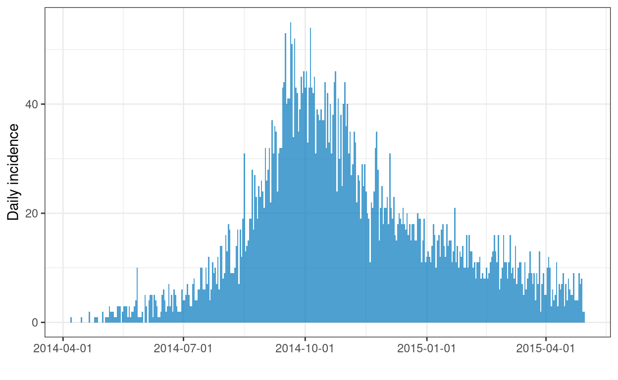
# a quick visualising the daily onsets
dat |> incidence(date_of_onset) |> plot()
# calculate the epiweek incidence across hospitals and plot
dat |>
  incidence(
    date_index = date_of_onset,
    groups = hospital,
    interval = "epiweek",
    na_as_group = FALSE
  ) |>
  print() |>
  facet_plot(nrow = 3, color = "white")
An incidence object: 262 x 3
date range: [2014-W15] to [2015-W17]
cases: 4373
interval: 1 (Sunday) week

   date_index hospital                                     count
       <yrwk> <fct>                                        <int>
 1   2014-W15 Military Hospital                                1
 2   2014-W16 Connaught Hospital                               1
 3   2014-W17 other                                            3
 4   2014-W18 Connaught Hospital                               1
 5   2014-W18 Princess Christian Maternity Hospital (PCMH)     1
 6   2014-W18 Rokupa Hospital                                  1
 7   2014-W19 Connaught Hospital                               3
 8   2014-W19 Military Hospital                                4
 9   2014-W19 other                                            1
10   2014-W19 Princess Christian Maternity Hospital (PCMH)     1
# … with 252 more rows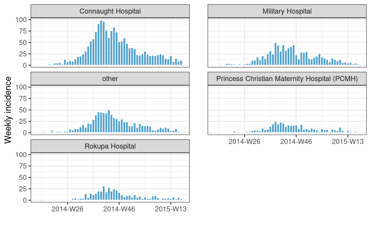
Example 2 - Pre-aggregated data
# get the data and filter out the nations
dat <- get_regional_data(country = "UK", verbose = FALSE)
nations <- c("England", "Northern Ireland", "Scotland", "Wales")
dat <- subset(dat, !region %in% nations)

# calculate iso-weekly new cases across regions and plot
dat |>
  incidence(
    date_index = date,
    counts = cases_new,
    groups = region,
    interval = "isoweek",
    na_as_group = FALSE
  ) |>
  print() |>
  facet_plot(angle = 45, n.breaks = 6)
An incidence object: 693 x 3
date range: [2020-W05] to [2021-W28]
cases_new: 4509597
interval: 1 (Monday) week

   date_index region                   cases_new
       <yrwk> <chr>                        <dbl>
 1   2020-W05 East Midlands                    0
 2   2020-W05 East of England                  0
 3   2020-W05 London                           0
 4   2020-W05 North East                       0
 5   2020-W05 North West                       0
 6   2020-W05 South East                       0
 7   2020-W05 South West                       0
 8   2020-W05 West Midlands                    0
 9   2020-W05 Yorkshire and The Humber         1
10   2020-W06 East Midlands                    0
# … with 683 more rows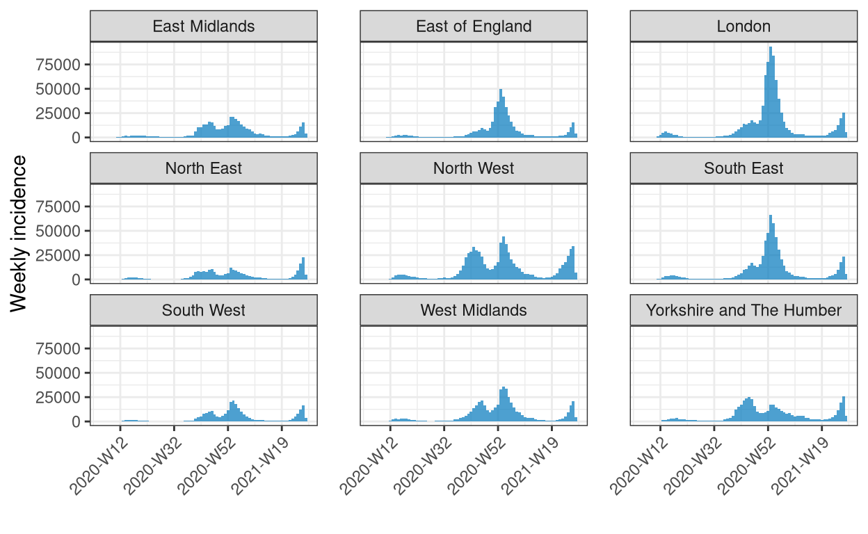
Final thoughts
Hopefully this short post gave you a taster of what incidence2 is about and why it is useful. For more information, including details on manipulating incidence objects, customizing the default plots, and using custom functions for date grouping, I recommend consulting the vignettes distributed with the package:
vignette("Introduction", package = "incidence2")vignette("handling_incidence_objects", package = "incidence2")vignette("customizing_incidence_plots", package = "incidence2")vignette("alternative_date_groupings", package = "incidence2")
Jombart, Thibaut, Simon Frost, Pierre Nouvellet, Finlay Campbell, and Bertrand Sudre. 2020. Outbreaks: A Collection of Disease Outbreak Data. https://CRAN.R-project.org/package=outbreaks.
Kamvar, Zhian N., Jun Cai, Juliet R. C. Pulliam, Jakob Schumacher, and Thibaut Jombart. 2019. “Epidemic Curves Made Easy Using the R Package Incidence.” F1000Research 8 (January): 139. https://doi.org/10.12688/f1000research.18002.1.
Müller, Kirill, and Hadley Wickham. 2021. Tibble: Simple Data Frames. https://CRAN.R-project.org/package=tibble.
Palmer, Joseph, Katharine Sherratt, Richard Martin-Nielsen, Jonnie Bevan, Hamish Gibbs, Sebastian Funk, and Sam Abbott. 2021. “Covidregionaldata: Subnational Data for Covid-19 Epidemiology.” Journal of Open Source Software 6 (62): 3290. https://doi.org/10.5281/zenodo.3957539.
Taylor, Tim. 2021a. Grates: Grouped Date Classes. https://CRAN.R-project.org/package=grates.
———. 2021b. Incidence2: Compute, Handle and Plot Incidence of Dated Events. https://CRAN.R-project.org/package=incidence2.
structural information that must remain true for an object to maintain its class when operated on↩︎